Examples of numerical semi-continuous functions

Though we have been previously discussing the abstract definition of lower and upper semi-continuity, there are also tailored definitions for numerical functions, single-valued multifunctions which map into the extended real numbers. For the moment, let’s only consider these numerical functions \(\newcommand{\set}[1]{\{#1\}} \renewcommand{\bar}{\overline} \newcommand{\RR}{\mathbb{R}} f : X \to \bar{\RR}\). The relevant sets for lower and upper semi-continuity become

\[\begin{align} \mathcal{L}_f(\lambda ; H ) &= \set{ x \in X : f(x) \leq \lambda} \\ \mathcal{U}_f(\lambda ; H ) &= \set{ x \in X : f(x) \geq \lambda}. \end{align}\]

These are just the normal level sets of \(f\). Since we will usually consider the cases when \(H = X\), let’s agree to the shorthand notations of \(\mathcal{L}_f(\lambda) = \mathcal{L}_f(\lambda ; X )\) and \(\mathcal{U}_f(\lambda) = \mathcal{U}_f(\lambda ; X )\).

Examples

The first basic (yet important) example of a function \(f : X \to \RR\) which is semi-continuous but not continuous is a step function:

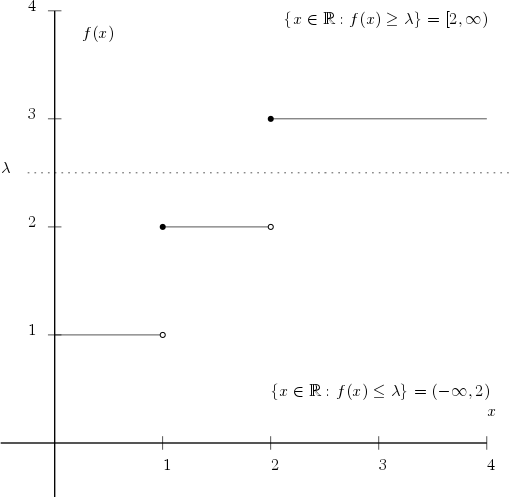
Here \(f : \RR \to \RR\) is defined by

\[f(x) = \begin{cases} 1 & x < 1 \\ 2 & 1 \leq x < 2 \\ 3 & 3 \geq x \end{cases}\]

I drew an arbitrary \(\lambda\) at around \(5/2\) to illustrate how semi-continuity works. In this case, \(\mathcal{L}_f(\lambda) = (-\infty, 2)\) is an open set, and in particular it is not closed. So we can see that \(f\) is not \(\RR\)-lower semi-continuous. However, \(\mathcal{U}_f(\lambda) = [2, \infty)\) which is closed. It seems to suggest that \(f\) may indeed by \(\RR\)-upper semi-continuous. Indeed, you can imagine sweeping the \(\lambda\) line up and down the plot, and no matter where it lands, the upper level set will be a closed set.

Why is this the case? We have to pay special attention to two facts. First, note that \(f\) is monotonically increasing. Second, notice how the jump discontinuities at \(1\) and \(2\) are oriented. In particular, the left-side limit of \(f\) does not match its actual value at these spots, whereas the right-side limit does. This means that if you swept \(\lambda\) down from \(+\infty\) and reached past, say, \(\lambda = 3\), the upper level sets have already gobbled up \((2,f(2))\), which is a limit point of the graph. As a consequence, the lower level sets will periodically miss limit points, violating closure.

Monotonicity is important for step functions to retain semi-continuity, but the direction matters for the specifics. In our case, \(f\) monotonically increases, and together with the arrangement of jump discontinuities gives us upper semi-continuity. If we considered \(-f\), which now monotonically decreases with the same jump discontinuities, it follows that \(-f\) is lower semi-continuous. Or, if we switched the arrangement of jump discontinuities for \(f\), then it would become lower semi-continuous. (Doing both exchanges returns us back to upper semi-continuity.)

For probability theory, distribution functions are always oriented like \(f\) in that they are monotonically increasing and upper semi-continuous.

Thomae’s function

Taking off the training wheels, let’s consider Thomae’s function, which is notorious in introduction to analysis courses. This is defined \(f : \RR \to [0,1]\) in the following way. If \(x \in [0,1]\) is irrational, then set \(f(x) = 0\). Otherwise, let \(x = p/q\) be the canonical rational form (that is, such that \(\gcd(p,q) = 1\), since there is only one such pair \((p,q)\)), and set \(f(x) = 1/q\). You get something which looks like the following plot¹:

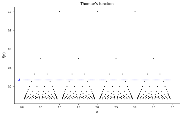
This is a function which is continuous at any irrational number but discontinuous at every rational number. I won’t prove this fact here. On \(\RR\), the entire function is clearly not continuous, but we might ask whether it is semi-continuous.

We’ll start with upper semi-continuity. So, let \(\lambda \in [0,1]\) be arbitrary. Notice that by definition \(\mathcal{U}_f(0) = \RR\), so consider the case when \(\lambda > 0\). To see that \(\mathcal{U}_f(\lambda)\) is closed, we will show that it has no limit points.² Let \(Q = \max \set{q \in \mathbb{N} : 1/q > \lambda }\),³ and let

\[\Delta = \inf \set{ |x-y| : x, y \in \mathcal{U}_f(\lambda)}.\]

Now, \(\mathcal{U}_f(\lambda)\) if and only if \(\Delta = 0\). Now at first glance, there’s no reason to suspect \(\Delta\) to be positive. But examine the plot again, and it starts to become clear that there are only finitely many different “widths” in the upper level set. Indeed, we actually have

\[\Delta = \inf \set{ |1/q - 1/q'| : q,q' \in \set{1,\dots,Q}, q \ne q' }.\]

But since the set on the right hand side has at most \(Q^2\) members, we can exchange the infimum for a minimum and conclude that \(\Delta > 0\). So \(\mathcal{U}_f(\lambda)\) has no limit points, and is vacuously closed. Hence, \(f\) is \(\RR\)-upper semi-continuous.

Of course, this also means that \(\mathcal{L}_f(\lambda)\) is not closed for any \(\lambda < 1\), which implies that \(f\) is not \(\RR\)-lower semi-continuous.

Endnotes

Published on June 27th, 2018 by David Kraemer